Let's set the scene¶

You're a researcher doing numerical modelling. You're an old hand. You use Python (and therefore are awesome).

Your days are spent constructing mathematical models, implementing them in code, and exploring the models as you change different parameters. You realize that simplicity is key, so you make sure to write your models as pure functions of the parameters, maybe a little something like this:

def complicated_model(x, y):
    ...
    return result

Beautiful; now it's time to do some science! Of course, you'll want to plot your model as a function of the parameters. Python makes this super simple but, as we'll see, this simplicity has a price.

You start off the same way you have a million times before: gridding your parameter space and mapping complicated_model over it:

N = 25
xs = np.linspace(-1, 1, N)
ys = np.linspace(-1, 1, N)

answers = [complicated_model(x, y) for x, y in itertools.product(xs, ys)]

Two minutes later (those simulations are heavy beasts!) and you realize you've massively underestimated the number of points you're going to need; you can't make out any detail at all! let's try that again.

N = 50
xs = np.linspace(-1, 1, N)
ys = np.linspace(-1, 1, N)

answers = [complicated_model(x, y) for x, y in itertools.product(xs, ys)]

Sure, you could probably incorporate the points from the previous run into this one – you are a numpy wizard after all – but in the time it would take you to get it right you could have just re-run the simulation anyway. Much more sensible to just change N to 50 and take a ten-minute coffee break waiting for the results.

Aww yes, a marginally improved plot! Let's hope you never want any more detail, or we could be here for quite a long time.

Sound familiar?¶

In our research group we found ourselves doing the above approximately fifteen quintillion times a day. That's why one day we got fed up and decided to write adaptive, a Python library for adaptive sampling (see what we did there?).

Using adaptive, you turn this:

N = 25
xs = np.linspace(-1, 1, N)
ys = np.linspace(-1, 1, N)

answers = [complicated_model(x, y) for x, y in itertools.product(xs, ys)]

into this:

def complete_when(learner):
    return learner.npoints >= 25**2

learner = adaptive.LearnerND(complicated_model, ((-1, 1), (-1, 1)))
adaptive.runner.simple(learner, complete_when)

The plot produced using adaptive uses the same number of points as the previous plot (625), but we get way more detail because it sampled more on the interesting ring, rather than the boring flat part.

If the above example has left you awestruck and ravenous for more, then read on!

Adaptive¶

In a nutshell adaptive's job is to simplify sampling functions over parameter spaces; it is useful when you don't care how your parameter space is sampled, just that it's sampled well. It will try its best to zoom in on the interesting regions, while making sure that seemingly "uninteresting" regions are not hiding any secrets. adaptive will also take advantage of multiple cores on your machine (using the power of concurrent.futures) or on remote machines (via ipyparallel or distributed).

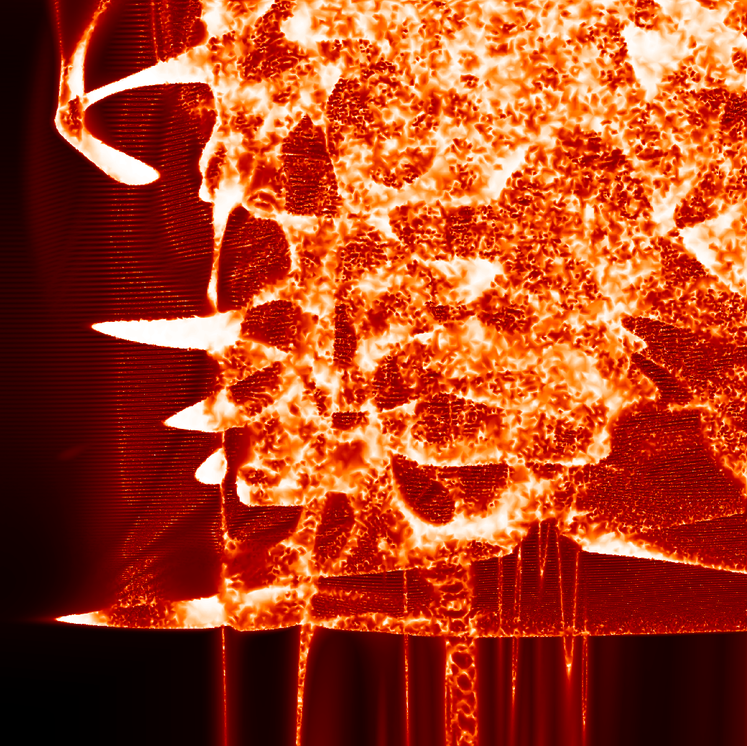
It is used extensively in the Quantum Tinkerer research group in TU Delft to run quantum transport simulations and create gnarly plots:

How can I get some of this hotness?¶

adaptive is developed on Github, and has packages available on PyPI and Conda Forge.

The easiest way to install adaptive is with

conda install -c conda-forge adaptive

Alternatively, if you use pip, then you can

pip install adaptive[notebook]

The [notebook] will make sure that you get all the goodies for notebook integration (adaptive works great as part of iterative, interactive workflows in the Jupyter notebook).

We also have a tutorial and documentation available on readthedocs.

A small disclaimer¶

Adaptive is pre- version 1.0, and we're still figuring out some interface stuff; don't be surprised if things break when you upgrade to a more recent version. That being said, adaptive has been successfully used in a number of research projects, and is actively developed, so if something doesn't work be sure to open an issue.

The core workflow¶

When using adaptive you'll create a Learner, providing the function to "learn", and the bounds on the domain of f.

import time
import adaptive

def f(xy):
    x, y = xy
    a, d = 0.2, 0.6
    time.sleep(0.005)  # do some hard work!
    return x + np.exp(-(x**2 + y**2 - d**2)**2 / a**4)

learner = adaptive.LearnerND(f, bounds=((-1, 1), (-1, 1)))

You can then ask this learner what points x you should evaluate next. Then it's up to you to evaluate your f on those points and tell adaptive about what values, f(x), are at those points.

# 'ask' also tells us how "important" the learner expects
# each point to be, but we ignore it here.
xs, _ = learner.ask(10)

for x in xs:
    learner.tell(x, f(x))

This is the same idea as the ask and tell from scikit-optimize. In fact, because adaptive doesn't say much about what Learners must do, beyond implementing ask and tell, Learners can implement whatever strategy they like to predict where the "best" place is for the next points.

Typically when using adaptive you won't call ask and tell yourself; you'll create a Runner that will ask the learner for as many points as it can evaluate at a time, and then run your function on any computational resources you declare. You can also give the Runner a goal, which tells it when to stop.

runner = adaptive.Runner(learner,
                         goal=lambda learner: learner.npoints >= 1000)

When using adaptive in a Jupyter notebook, the Runner will do its job in the background. This means that you can get live information about its progress, as well as live-plotting data as it is produced. This is awesome for interactive workflows.

# run once to enable live info and plotting
adaptive.notebook_extension()

runner.live_info()
runner.live_plot(update_interval=0.1)

But how does it work?¶

I said above that we modelled the core Learner API after scikit-optimize, however in practice the Learners that we have implemented so far are not based on Bayesian optimization (although we would welcome pull requests!)

In practice the learners implemented so far all work in more or less the same way:

Divide the function domain into subdomains (intervals in 1D, triangles in 2D etc.), and put points at the corners
Define a loss function over each subdomain
Sort the subdomains by their loss
When asked for more points, select the subdomains with the largest losses, bisect them, and add points at the corners of the newly added subdomains

It's illustrative to look at the algorithm in 1D to see how this works.

You can use the slider below to add points; the red line and red points indicate the interval with the largest loss. If you increase the number of points by 1, the learner will place a point in the center of the red interval (bisecting it) and the interval with the next-largest loss will be marked in red.

Decomposing the problem in terms of subdomains and loss functions is useful for a couple of reasons: it's cheap, and it's easily parallelizable.

Because the loss function is local – it depends only on a single subdomain and perhaps its neighbours – it costs $O(1)$ to compute for new subdomains, and $O(\log N)$ to insert into the priority queue of subdomains. This means that sampling $N$ points should take $O(N \log N)$ time. The easy parallelism comes from simply asking for $n$ points at a time, where $n$ is matched with the available computational resources.

In practice these two properties mean that the Learners implemented in adaptive are very effective for plotting and interactive exploration.

What loss function do you use?¶

In the first few sentences of this article I said:

We don't care about how points are sampled, just that they're sampled well

but how do we define "well-sampled"? It's largely a matter of opinion. Perhaps you really care about regions where your function is steep, or only where the slope changes rapidly. Maybe you want to guarantee that features of a certain size will definitely be captured, or maybe you don't really care about the details, and just want something that "looks good" when plotted.

With the Learner implementation I introduced in the last section we can choose what "well-sampled" means for us by choosing a loss function. By constructing a loss function that is large on regions that we consider "interesting" we can guide the algorithm to prefer these regions.

The Learners implemented in adaptive leave the choice of loss function up to you, however we also provide a simple default that seems to work pretty well in practice (all of the examples in this post use the default loss). The process of designing a good loss function is worth a whole blog post by itself, so for now we'll just say what the default is and save the lengthy explanations for later.

The default loss we use is the simplest thing that could possibly work: the distance in the plane between neighboring points.

That's it. I was pretty astounded that this would produce intelligible results, but it does a stellar job, given its simplicity. Another advantage of using this loss function as a default is that it trivially extends to higher-dimensional domains domains and codomains: for a function $\;f : ℝ^n \to ℝ^m$ the default loss corresponds to the volume of the $n$-simplex defining a subdomain (line, triangle, tetrahedron in 1D, 2D and 3D respectively) embedded in $n+m$ dimensional space.

Recently we've also been tinkering with alternate loss functions, which we may use as the default in the future. One particularly neat idea is to use a "reverse" Visvalingam Whyatt algorithm (RVW), where we assign loss based on the area of the triangles "associated" with the interval. The figure below should give you the gist of the idea:

This loss has the advantage that it prioritizes changes in slope, rather than just steep regions, so it will zoom in on features that "stick out". On the other hand, it will penalize very abrupt and isolated changes, so won't get stuck on discontinuities as much as the distance-in-the-plane loss function.

Where we're going¶

Adaptive is a work in progress, and there are a few areas where I'd like to see us improve in the coming months.

Experimental control¶

The main area where I'd like to see adaptive become more powerful is in controlling physics (or other) experiments. Maybe you've got some circuit attached to a voltage source and an electromagnet, and you want to measure the current flowing through the circuit for different voltages and magnetic fields. Instead of sweeping the parameters manually, we'd like to hand the reins to adaptive and have it control the experiment for us. In my opinion adaptive sampling can transform how experiments are done, especially in my own domain of quantum nanoelectronics. With that possibility comes a metric tonne of of new challenges to overcome. For one, jumping around in parameter space is just fine and dandy when you're doing a simulation, but if you suddenly crank your electromagnet up to 5 Tesla you're going to have a bad time. There's also the joy of dealing with hysteresis, where you have to care not only where you are in parameter space but how you got there too.

Better abstractions¶

We'd like to make adaptive more composable and extensible, so that it can be used in ways that we haven't even thought of yet. While dogfooding adaptive within our research group we found ourselves bolting on bits and pieces as we needed: easy saving/loading of data from previous runs, having functions return metadata (e.g. runtime) in addition to results, balancing resources between several learners based on their loss, etc. Our approach while adding these pieces was "if it solves our immediate problem, we'll add it". This is because it's really hard to know how to make something extensible if you have no idea in what direction you'd like to extend it. By progressively adding features that "get the job done", but without thinking too hard how everything fits together as a whole, we've managed to accumulate a body of use-cases. Now I'd like to see us use that data to make a cleaner and more ergonomic interface to adaptive.

How you can help¶

Give it a try!¶

If you think you'd find adaptive useful, please give it a try! We are very interested in hearing about different use cases, and suggestions about how we can make adaptive even more awesome. You can install adaptive right now by opening a terminal and typing

conda install -c conda-forge adaptive

pip install adaptive[notebook]

Get involved!¶

If you'd like to get involved with developing adaptive further, that would be awesome. We're on on Github, so get yourself over there to open an issue or a pull request!